
RAG Evaluation Metrics
Introduction & Overview
Retrieval Augmented Generation (RAG) is the process of enhancing a language model’s responses by retrieving relevant information from an external knowledge source—such as documents, databases, or web pages—and using that information to generate more accurate, context-aware outputs. Evaluating RAG systems requires assessing multiple factors, starting with how effectively they retrieve relevant information (Retrieval Metrics) and the quality of the text they generate using approaches like BLEU or ROUGE (Generation Metrics). Beyond basic retrieval and generation, evaluation delves into the nuances of response relevance, factual faithfulness (including checks like HHEM), and semantic similarity (using methods like BERTScore or SEM Score). Ultimately, assessment combines automated techniques, from simple string matching to sophisticated LLM-based evaluations like G-Eval, with the crucial insights gained from human judgment. The overarching goal of developing and utilizing these diverse metrics is to create reliable proxies that automate or simulate the comprehensive and nuanced assessments typically performed by human evaluators.
Retrieval Metrics
How well does the system retrieve useful documents?
Retrieval evaluation metrics are essential tools for measuring and improving the performance of information retrieval systems such as search engines, recommendation systems, and question-answering platforms. These metrics help quantify how effectively a system can retrieve relevant information in response to user queries.
The choice of evaluation metric significantly impacts how we perceive system performance and guide development efforts. No single metric is universally ideal—different scenarios call for different evaluation approaches based on user needs, application context, and available resources.
Why Retrieval Metrics Matter
Retrieval metrics matter for several critical reasons:
- Performance Measurement: They provide objective ways to measure how well retrieval systems perform at their fundamental task.
- System Comparison: They enable meaningful comparisons between different retrieval approaches or algorithms.
- Optimization Guidance: They offer signals for what aspects of a system should be improved and can guide algorithmic refinements.
- User Experience Alignment: The right metrics can align closely with actual user satisfaction and experience quality.
- Business Impact: Improvements in these metrics often translate directly to business outcomes like increased user engagement or conversion rates.
Variants of Retrieval Metrics
Retrieval metrics broadly fall into two major categories — Binary (relevant or not) and Graded (relevance can have multiple levels) — each with distinct subcategories based on how they treat relevance and result ordering.
Binary Relevance Metrics treat documents as either relevant or non-relevant to a query, without intermediate degrees of relevance.
Order-Unaware Binary Metrics only consider whether relevant documents are retrieved, regardless of their position in results: Precision, Recall, F1 Score. Order-unaware metrics are suitable when all retrieved results are presented simultaneously (as in a set) or when position doesn’t significantly affect the likelihood of user interaction.
Order-Aware Binary Metrics account for both relevance and the position of documents in the result list: Mean Reciprocal Rank (MRR, Focuses on the position of the first relevant result), Mean Average Precision (MAP, Averages precision values at positions where relevant documents appear). Order-aware binary metrics are appropriate when users typically scan results sequentially from top to bottom, making position crucial to discovery probability.
Graded Relevance Metrics recognize that relevance exists on a spectrum rather than as a binary state. Documents can be partially relevant, highly relevant, or somewhere in between:
Discounted Cumulative Gain (DCG): Accumulates graded relevance scores with a position-based discount
Normalized DCG (NDCG): Normalizes DCG to enable cross-query comparisons
Expected Reciprocal Rank (ERR): Models user behavior as a cascade process considering both relevance grades and position
Graded relevance metrics provide more nuanced evaluation, particularly valuable in domains where relevance naturally exists on a spectrum rather than as an all-or-nothing property.
Further Reading:
- Metrics for Evaluation of Retrieval in Retrieval-Augmented Generation (RAG) Systems
- Evaluating RAG Part I: How to Evaluate Document Retrieval
- Evaluation Metrics for Retrieval Augmented Generation (RAG) Systems
- Ultimate Guide to Evaluate RAG System
- RagEval: Scenario-Specific RAG Evaluation Dataset Generation Framework
- RAG-QA Arena: Evaluating Domain Robustness for Long-form Retrieval Augmented Generation
Selecting Appropriate Metrics
The choice of evaluation metric should be driven by:
- User Behavior: How users interact with search results (scan depth, tolerance for irrelevance)
- Task Nature: Whether completeness (recall) or precision is more important
- Result Presentation: Whether results are ranked, paginated, or presented simultaneously
- Relevance Complexity: Whether relevance is naturally binary or multi-faceted
- Available Judgments: What kind of relevance assessments are available or feasible to obtain
Understanding these categories helps inform which metrics best align with specific retrieval systems and use cases. The following sections will explore each metric in detail, providing formal definitions and practical examples. Now let’s look at the specific evaluation metrics.
1. Precision@k
Precision@k measures how many of the top-k retrieved documents are actually relevant to a user’s query. Think of it as measuring the quality or accuracy of your top results. For example, if a search engine returns 10 documents (k=10) and 7 of them are relevant to your query, the Precision@10 would be 7/10 = 0.7 or 70%. This metric is particularly useful in scenarios where users typically only look at a limited number of search results, like the first page of a web search. A high Precision@k indicates that users can trust the top results they’re seeing.
BLEU and METEOR
- Definition: The proportion of retrieved documents in the top-k results that are relevant
- Formula: Precision@k = (# of relevant documents in top k) / k
- Use case: Measures retrieval quality when users only care about a fixed number of top results
- Strengths: Easy to understand and calculate; focuses on quality of top results
- Limitations: Doesn’t account for total number of relevant documents in corpus
2. Recall@k
Recall@k evaluates how many of all possible relevant documents in the entire database were successfully captured in the top-k results. It focuses on completeness rather than accuracy. For instance, if there are 20 documents in a database that would be relevant to a particular query, and a search engine returns 10 results (k=10) containing 5 of those relevant documents, the Recall@10 is 5/20 = 0.25 or 25%. Recall becomes crucial in applications like legal document discovery or medical research, where missing relevant information could have serious consequences.
- Definition: The proportion of all relevant documents that are retrieved in the top-k results
- Formula: Recall@k = (# of relevant documents in top k) / (total # of relevant documents)
- Use case: Important when finding all relevant items is critical (e.g., legal discovery)
- Strengths: Measures completeness of retrieval
- Limitations: Can be gamed by returning many documents; requires knowing all relevant documents
3. F1@k
F1@k provides a balanced approach by combining both Precision@k and Recall@k into a single metric using the harmonic mean. This addresses the inherent trade-off between precision and recall. For example, if a system has a Precision@10 of 0.7 (70% of retrieved documents are relevant) and a Recall@10 of 0.5 (retrieved 50% of all relevant documents), the F1@10 would be 2 × (0.7 × 0.5) ÷ (0.7 + 0.5) = 0.583. F1@k is valuable when you need a system that’s both accurate and thorough, without sacrificing too much of either quality.
- Definition: Harmonic mean of Precision@k and Recall@k
- Formula: F1@k = 2 × (Precision@k × Recall@k) / (Precision@k + Recall@k)
- Use case: Balances precision and recall when both are important
- Strengths: Single metric capturing both precision and recall
- Limitations: Treats precision and recall as equally important
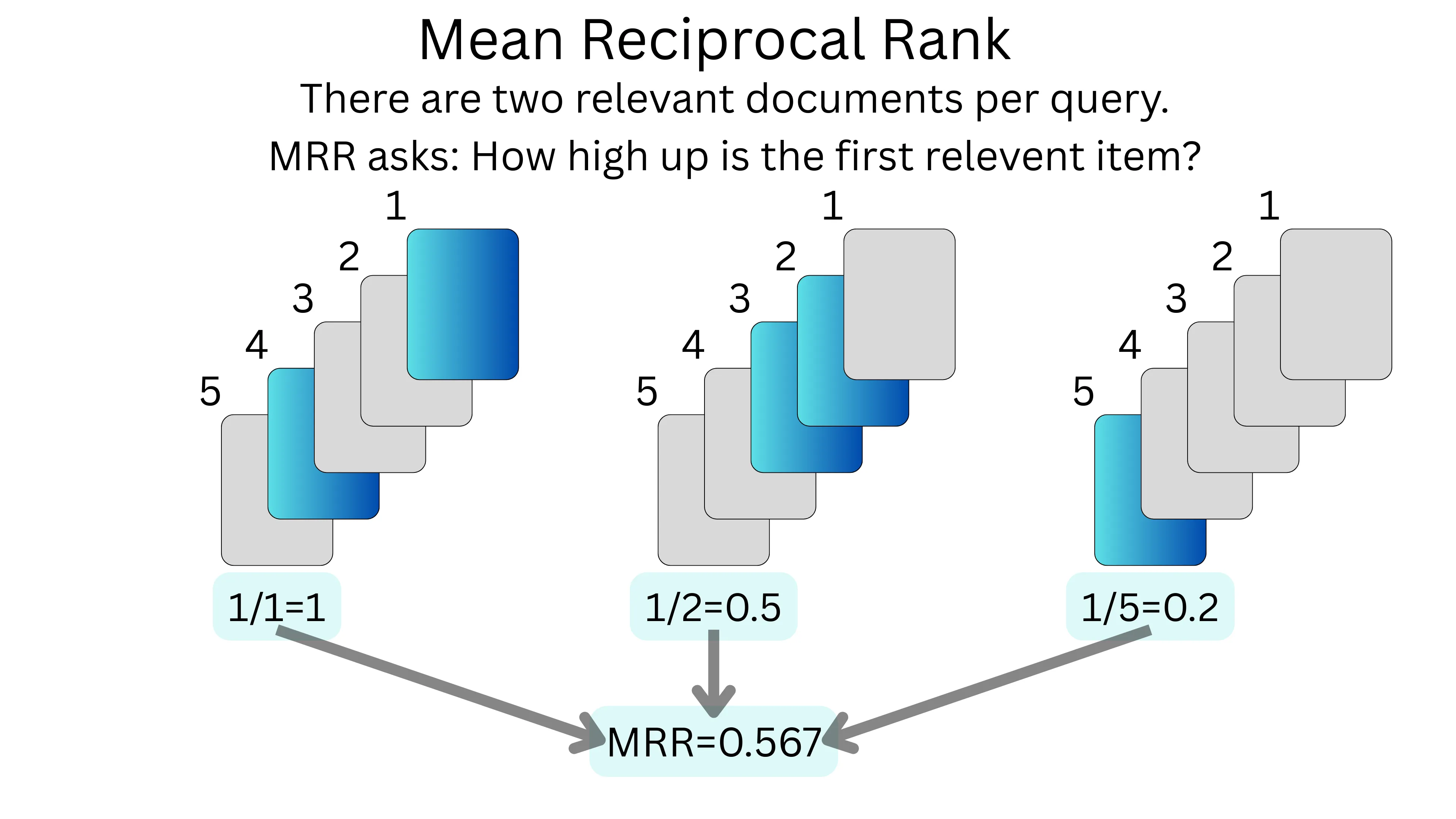
4. Mean Reciprocal Rank (MRR)
MRR focuses on how quickly a retrieval system finds the first relevant document, which is perfect for question-answering systems where users want an immediate correct answer. It calculates the average of the reciprocal of the rank at which the first relevant document appears. For example, if for three different queries, the first relevant document appears at positions 1, 2, and 5 (as seen in the image below) respectively, the MRR would be (1/1 + 1/2 + 1/5) ÷ 3 = 0.567. A higher MRR indicates that the system typically places relevant results at or near the top of the list.
-
Definition: Average of reciprocal ranks of the first relevant document across queries
-
Formula:
- U = Total number of users or queries.
- u = Index over users or queries (from 1 to U).
- rankᵢ = Rank position of the first relevant (or correct) item for the i-th user or query.
-
Use case: When only the first relevant result matters (e.g., question answering)
-
Strengths: Simple single-number metric; emphasizes getting at least one relevant result early
-
Limitations: Ignores relevant documents after the first one
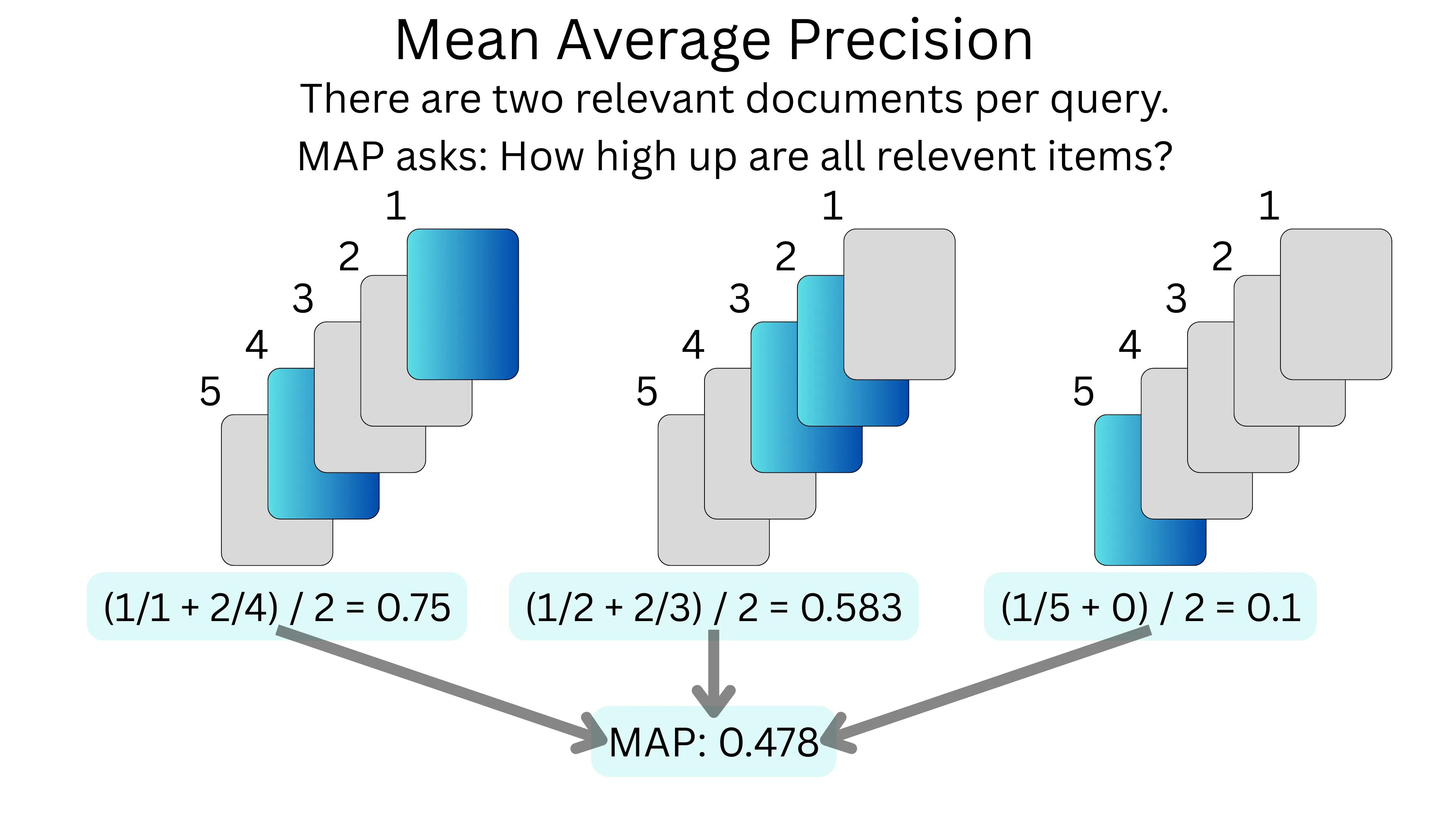
5. Mean Average Precision (MAP)
MAP provides a comprehensive evaluation by averaging the precision values calculated after each relevant document is retrieved. Consider a query where relevant documents appear at positions 1, 3, and 7 in a list of 10 results. The precision at each relevant position would be 1/1, 2/3, and 3/7. The average precision for this query would be (1 + 2/3 + 3/7) ÷ 3 = 0.81. MAP is then calculated by averaging these values across multiple queries. This metric rewards systems that rank relevant documents higher and is widely used in information retrieval evaluation campaigns.
- Definition: Mean of Average Precision scores across all queries
- Formula:
Where:
- Use case: Comprehensive evaluation of ranked retrieval systems
- Strengths: Considers both precision and ranking quality; robust summary metric
- Limitations: More complex to calculate; all relevant documents must be known
6. Discounted Cumulative Gain@k (DCG@k),
Normalized **Discounted Cumulative Gain@k (NDCG@k)
Discounted Cumulative Gain (DCG@k) and its normalized version (NDCG@k) are sophisticated metrics that account for both the relevance level of documents and their positions. Unlike binary relevance used in previous metrics, these can handle graded relevance (e.g., highly relevant, somewhat relevant, not relevant). For instance, if documents with relevance scores [3, 2, 0, 1, 0] appear in that order, the DCG@5 would sum these values with logarithmic position discounts: 3 + 2/log₂(3) + 0 + 1/log₂(5) + 0 = 4.63. NDCG@k normalizes this value by dividing by the “ideal” DCG, making it possible to compare performance across different queries with varying numbers of relevant documents.
-
Definition:
- DCG@k: Discounted Cumulative Gain, measures relevance with position discount
- NDCG@k: Normalized DCG, divides DCG by ideal DCG
-
Formula:
- K is the rank cutoff — it specifies how many of the top-ranked items you’re evaluating.
- k = Current position in the ranking (from 1 to K).
- relₖ = Relevance score of the item at position k.
- log₂(k + 1) = Logarithmic discount factor (we use k + 1 to avoid division by zero).
- DCG@K = Discounted Cumulative Gain at rank K (from above).
- IDCG@K = Ideal Discounted Cumulative Gain at rank K (this is the DCG of the best possible ranking — i.e., items ranked in perfect order of relevance).
In short:
- DCG@K measures the gain of your ranking, discounted by position.
- NDCG@K normalizes it by comparing to the ideal ranking, so it’s between 0 and 1 (higher is better).
-
Use case: When documents have graded relevance and ranking quality matters
-
Strengths: Accounts for position and graded relevance; normalized version allows cross-query comparison
-
Limitations: Requires relevance judgments on a scale rather than binary judgments
7. Expected Reciprocal Rank (ERR)
Expected Reciprocal Rank (ERR) is a sophisticated retrieval metric that models user behavior as a cascade process, where users scan results from top to bottom and may stop once they find sufficiently relevant information. Unlike metrics that assume users examine all results, ERR accounts for the probability that a user’s information need is satisfied at each position. For example, with documents of relevance scores [3, 2, 0, 1, 0] on a 0-3 scale, ERR calculates the expected stopping position based on the probability that each document satisfies the user, giving more weight to finding highly relevant documents early in the ranking.
- Definition: Expected Reciprocal Rank, models the expected reciprocal length of time a user will spend searching
- Formula: depends on relevance of current and previous documents
- Use case: Web search evaluation where users typically stop after finding satisfactory information
- Strengths: Models realistic user behavior; accounts for diminishing returns of multiple relevant documents; uses graded relevance
- Limitations: More complex to calculate; requires careful calibration of relevance grades to satisfaction probabilities
Generation Metrics
How well does the generated text match reference outputs?
Generation metrics are crucial for evaluating the quality of text generated by various models, providing an automated way to assess different aspects like how well the generated text matches reference text (using n-gram overlap in metrics like BLEU and ROUGE, or semantic similarity in BERTScore and SEM Score), how relevant and faithful it is to the input or source (measured by relevance and faithfulness metrics), and even its human-like qualities such as fluency and coherence (assessed by LLM-based evaluations like G-Eval). These metrics work by employing diverse techniques, ranging from simple word or character sequence comparisons to complex semantic understanding through embeddings and even leveraging the judgment capabilities of large language models, ultimately providing scores or classifications that help developers understand and improve their text generation systems.
With generation metrics, we prioritize assessing various aspects of generated text quality, such as accuracy, relevance, fluency, and coherence, depending on the specific application and desired characteristics. Crucially, many of these evaluations also take into account the retrieved documents or data used to generate the text, assessing how well the generated output is grounded in and consistent with this source material.
Traditional — N-gram Matching Approaches
An n-gram is a contiguous sequence of n words or characters in a text. In BLEU, ROUGE, and METEOR, n-grams are used to compare generated text to a reference:
- BLEU: Measures precision of overlapping n-grams between candidate and reference.
- ROUGE: Focuses on recall, counting how many reference n-grams appear in the candidate.
- METEOR: Uses harmonized precision, recall, and synonym matching on n-grams for better semantic evaluation
BLEU (Bilingual Evaluation Understudy)
What is BLEU?
BLEU (Bilingual Evaluation Understudy) is a metric originally designed to assess the quality of machine translation systems. It quantitatively measures how much a candidate (or generated) translation overlaps with one or more reference translations.
How Does BLEU Work?
BLEU compares n-grams between the candidate translation and the reference translation(s). The key processes involved are:
-
n-gram Precision: BLEU counts the matching sequences of words—called n-grams—for different values of n (typically 1, 2, 3, and 4). For each n-gram, the number of overlapping n-grams is compared against the reference. Clipping is applied so that a candidate does not receive extra credit for repeating n-grams more times than they appear in the reference. Here, the numbers 1, 2, 3, and 4 refer to the character/word count of each chunk.
-
Geometric Mean of Precisions: Higher-order n-gram matches (like bigrams, trigrams, etc.) become exponentially rarer. BLEU combines all the n-gram precision scores using the geometric mean, often computed via logarithms to appropriately weigh each precision value.
-
Brevity Penalty (BP): To discourage candidate translations from being overly short—an issue that could artificially boost precision—a brevity penalty is applied. The BP is calculated as:
This factor reduces the final score if the candidate translation is significantly shorter than the reference.
The Formula
The final BLEU score is the product of the geometric mean of the n-gram precisions and the brevity penalty. In mathematical notation, this is expressed as:
Where:
- pₙ is the precision for n-grams of length n (for example, unigram, bigram, trigram, and 4-gram).
- wₙ are the weights assigned to each n-gram level (typically equal weights, e.g., 1/4 each when using up to 4-grams).
- BP is the brevity penalty that adjusts the score for translations that are shorter than the reference.
This formulation helps ensure that BLEU captures both adequacy (through lower-order n-grams) and fluency (through higher-order n-grams), while discouraging translations that are incomplete.
Advantages
Popularity and Simplicity: BLEU is widely used because it is straightforward to compute and easy to interpret, making it a popular benchmarking tool for machine translation systems.
Objective Measurement: It provides an objective method to compare different translation models by quantifying the overlap between candidate and reference translations.
Limitations
Lack of Semantic Understanding: BLEU only considers surface-level n-gram matching. It does not capture the deeper semantic meaning of the text. For example, a candidate translation might score high even if it is factually incorrect:
- Candidate: “The Eiffel Tower is located in India.”
- Reference: “The Eiffel Tower is located in Paris.”
No Context or Fluency Adjustment: The metric does not account for the overall fluency or the contextual correctness of the translation; it solely focuses on word overlap.
Further Reading:
ROUGE (Recall-Oriented Understudy for Gisting Evaluation)
ROUGE (Recall-Oriented Understudy for Gisting Evaluation) is a set of metrics designed to evaluate automatic text summarization and machine translation systems. Developed by Chin-Yew Lin in 2004, ROUGE has become one of the standard evaluation methods in natural language processing, particularly for summarization tasks.
Core Concept: ROUGE fundamentally measures how much overlap exists between a machine-generated summary and one or more reference (human-written) summaries. Unlike BLEU, which focuses on precision, ROUGE was originally designed with recall in mind - measuring how much of the reference content is captured in the generated text.
It measures the extent to which words from the reference sentences are included in the generated sentence (capturing the idea of recall). It is good to use when working with text summarization tasks to automatically generate a concise summary of a longer text, where we want to capture the overall meaning.
ROUGE-N
ROUGE-N precision can also be calculated by replacing the denominator with the total count of n-grams in the generated summary.
This measures n-gram overlap between the system output and reference summaries. The formula for ROUGE-N recall is:
ROUGE-N = Count_match(gram_n) / Count(gram_n)
Where:
Count_match(gram_n)is the maximum number of n-grams co-occurring in the candidate summary and the reference summary.Count(gram_n)is the number of n-grams in the reference summary.
ROUGE-1: Measures individual word overlap to check if the generated text covers the important words from the reference.
ROUGE-2: Measures bigram overlap to capture short, meaningful phrase accuracy and local fluency.
ROUGE-L: Uses the longest common subsequence to evaluate sentence-level structure and the logical flow of words. The key advantage of ROUGE-L is that it considers sentence-level structure similarity rather than just n-gram overlap. The LCS doesn’t require consecutive matches but preserves word order, making it more flexible than strict n-gram matching.
ROUGE-S: Looks at skip-bigram pairs to detect flexible word pairings that maintain the correct order.
ROUGE-SU: Combines skip-bigrams with unigram overlap for a balanced evaluation of both individual words and flexible word pairs.
ROUGE-W: Builds on ROUGE-L by giving extra weight to consecutive word matches, rewarding more fluent and cohesive sequences.
Table 1: Different Varients of Rough
| Metric | Focus | Best For |
|---|---|---|
| ROUGE-1 | Word presence | General relevance |
| ROUGE-2 | Short phrases | Local fluency |
| ROUGE-L | Sequence order | Sentence structure, coherence |
| ROUGE-S | Flexible pairs | Order-aware paraphrasing |
| ROUGE-SU | Flexible + words | Hybrid balance |
| ROUGE-W | Weighted sequences | Rewarding longer exact matches |
Measurement Types
ROUGE can be calculated in three ways:
-
Recall: Measures how much of the reference summary is captured in the generated summary
R = Overlapping content / Reference content -
Precision: Measures how much of the generated summary appears in the reference summary
P = Overlapping content / Generated content -
F1-Score: The harmonic mean of precision and recall
F1 = (2 × P × R) / (P + R)
These formulas are not specific to one ROUGE variant, they apply to all of them. When you compute ROUGE, you first choose what kind of overlap you care about.
Multiple References
When multiple reference summaries are available, ROUGE typically calculates scores against each reference and takes either:
- The maximum score (optimistic approach)
- The average score (more balanced approach)
Example
Consider this example:
- Reference: “The Eiffel Tower is located in Paris.”
- Generated: “The Eiffel Tower is located in India.”
For ROUGE-1:
- Overlapping unigrams: “The”, “Eiffel”, “Tower”, “is”, “located”, “in”
- Reference unigrams: “The”, “Eiffel”, “Tower”, “is”, “located”, “in”, “Paris”
- Generated unigrams: “The”, “Eiffel”, “Tower”, “is”, “located”, “in”, “India”
ROUGE-1 Recall = 6/7 = 0.86
ROUGE-1 Precision = 6/7 = 0.86
ROUGE-1 F1 = 0.86
This example illustrates a key limitation: despite the factual error (placing the Eiffel Tower in India), ROUGE gives a high score because of the lexical overlap.
Advantages of ROUGE
- Correlates with human judgments: Multiple studies have shown reasonable correlation with human evaluations of summary quality
- Computationally inexpensive: Easy and fast to calculate
- Language-independent: Can be applied to summaries in any language
- Multiple variants: Different variants can capture different aspects of summary quality
Limitations
- Lexical focus: Cannot effectively capture semantic meaning or paraphrasing
- Limited syntactic insight: May not adequately assess grammatical correctness
- False positives: As shown in the example, can give high scores to factually incorrect content
- Reference dependence: Quality evaluation is limited by the quality and comprehensiveness of reference summaries
- Limited context understanding: Cannot evaluate if the most important information is included
Modern Developments and Usage
In practice, researchers often report multiple ROUGE variants (ROUGE-1, ROUGE-2, ROUGE-L) alongside other metrics to provide a more comprehensive evaluation. Additionally, rouge will be often combined with other evaluation methods including BERTScore, METEOR, and Human evaluation.
When implementing ROUGE:
- Consider stemming/lemmatization to handle morphological variants
- Decide how to handle stopwords (including or excluding them)
- Determine how to aggregate scores for multiple references
- Choose appropriate variants for the specific task (e.g., ROUGE-1 for general content overlap, ROUGE-2 for fluency, ROUGE-L for sequence alignment)
Further Reading:
METEOR (Metric for Evaluation of Translation with Explicit ORdering)
METEOR is an advanced metric used to evaluate the quality of machine translation outputs. Unlike other translation evaluation metrics, METEOR was specifically designed to address limitations in the popular BLEU metric and provide better correlation with human judgment, particularly at the sentence or segment level.
Core Concept: METEOR evaluates translations by creating alignments between a candidate translation (the machine output) and a reference translation (human-created standard). Its scoring system is based on a weighted harmonic mean of unigram precision and recall, with a notable emphasis on recall over precision. This weighting reflects the understanding that including all the correct information (recall) is often more important in translation than avoiding wrong information (precision).
METEOR incorporates several sophisticated matching techniques that distinguish it from other metrics:
- Exact matching - Identifies identical words between candidate and reference
- Porter stemming - Matches word variants with the same root (e.g., “good” and “goods”)
- WordNet synonymy matching - Recognizes semantic equivalents (e.g., “well” and “good”)
- Ordering consideration - Penalizes poor word order through alignment crossing
Algorithm Components
METEOR’s algorithm works through multiple stages and phases:
Mapping Stages
METEOR typically uses three consecutive mapping stages, each employing a different module:
- Exact module - Maps identical unigrams
- Porter stem module - Maps unigrams that share the same stem after applying the Porter stemmer
- WordNet synonymy module - Maps unigrams that are synonyms of each other
Phase 1: Identifying Unigram Mappings
In each stage, all possible unigram mappings are identified based on the current module. After the first stage, only previously unmapped unigrams are considered.
Phase 2: Selecting Optimal Alignment
When multiple possible alignments have the same number of mappings (cardinality), METEOR selects the alignment with the fewest “crosses” (intersections between mapping lines).
This can be determined:
- Visually by counting intersections in the mapping diagram
- Mathematically by calculating the number of crossing mappings

Phase 3: Score Calculation
Score = Fmean * (1-Penalty)
Fmean = 10PR / (R + 9P)
Penalty
Order of unigram pairings are considered through a penalty. Adjacent unigrams pairs are grouped into chunks as much as possible if they are adjacent in the response and reference. This results in # chunks = 1 if the response matches the reference. If there are no bigram or longer matches, then # chunks = # unigram matches
Penalty = 0.5 * (#chunks / #unigrams_matched)
The final METEOR score combines:
- Precision (P) = Number of unigrams mapped / Total unigrams in response (candidate)
- Recall (R) = Number of unigrams mapped / Total unigrams in reference
- Weighted Harmonic Mean (Fmean) = 10PR/(R+9P)
- This formula weights recall 9 times more heavily than precision
- Penalty for word order differences:
- Adjacent unigram pairs are grouped into chunks if they appear adjacently in both response and reference
- If the word order is perfect, chunk count = 1
- If there are no adjacent matches, chunk count = number of unigram matches
- The penalty is calculated based on these chunks to account for word ordering
Performance vs. BLEU
METEOR demonstrates significantly higher correlation with human judgments compared to BLEU:
- At corpus level: METEOR achieves correlation up to 0.964 vs. BLEU’s 0.817 on the same data (according to Wikipedia)
- At sentence level: METEOR reaches 0.403 correlation with human judgment (according to Wikipedia)
Practical Applications
METEOR is particularly valuable in:
- Evaluating translation systems where capturing meaning is more important than exact wording
- Research contexts requiring sentence-level translation quality assessment
- Scenarios where recall (completeness of information) matters more than precision
Further Reading:
- https://www.cs.cmu.edu/~alavie/papers/BanerjeeLavie2005-final.pdf
- https://en.wikipedia.org/wiki/METEOR
Faithfulness
Does the answer stay true to the retrieved or factual sources?
Faithfulness measures how factually consistent a response is with the retrieved context. This is useful in preventing hallucinations and ensuring the generation part of RAG is accuratly reflecting the retrieved data. Faithfulness is measured by the extent to which the claims are supported by the retrieved data.
Steps to measure fathfulness:
- Identify all claims in the response
- Check each claim to see if it can be inferred from the retrieved context
- Compute the faithfulness score
Faithfulness Score = Number of claims in the response supported by the retrieved context / Total number of claims in the response
HHEM (an option for step 2 of faithfulness)
This is the first evaluation model accepted as an industry standard for detecting hallucinations. Unlike methods that use a large language model (LLM) acting as a judge, this system is a pure classification model. By not relying on an LLM judge, it overcomes two major issues inherent in that approach:
- Performance and Cost: Using an LLM as a judge tends to be slow and expensive, which makes it unsuitable for real-world production environments that demand low latency.
- Overfitting Risks: In a judge-based approach, the same model (or a similar one) is used to assess the quality of generated outputs. Over time, this system may end up “listening” primarily to its own evaluations. If the initial judge has certain biases or tendencies, those biases can be continuously reinforced. In other words, if the judge consistently deems a particular style or error as acceptable, then the generation process can start mirroring those inaccuracies repeatedly. This cycle of self-reinforcement is what’s often referred to as an “echo chamber” effect.
Overfitting Explained
Definition in Context: Overfitting typically refers to a model learning the details and noise in its training data so well that it performs poorly on new, unseen data. In the context of judge-based methods, a similar concept applies—the model becomes overly tailored to its own evaluative criteria rather than learning a broader, more general set of high-quality responses.
Consequences of Overfitting: When a model is overfitting, it means it might be excelling in producing content that meets the internal judge’s expectations, but this “optimized” output might not generalize well to the varied demands of real-world scenarios or different contexts. The judge might reject innovative or unconventional answers simply because they fall outside of its narrow evaluative scope. In essence, the system risks losing flexibility and robustness.
The model’s effectiveness was evaluated by benchmarking it against GPT‑3.5 Turbo and GPT‑4, as well as against RAGAS (which itself incorporates these models), using two well-known hallucination benchmark datasets: AggreFact and RAGTruth. The result is that HHEM-2.1 outperforms GPT-3.5-Turbo and GPT-4. (source: https://www.vectara.com/blog/hhem-2-1-a-better-hallucination-detection-model)
Factual Correctness
Factual correctness measures the factual accuracy between generated response and reference.
This is achieved by using an LLM to breakdown response and reference into claims, then use natural language inference to determine the factual overlap between the response and the reference.
How its done
- Break Down into Claims: An LLM splits both the generated response and the reference text into individual factual claims.
- Compare Claims: Using natural language inference (NLI), the system determines if each response claim is:
- Supported by the reference (entailment)
- Contradicted by the reference (contradiction)
- Neither supported nor contradicted (neutral)
- Calculate Score: The system produces a score based on how many claims match between response and reference.
How Sentences Are Decomposed
Two key parameters control how sentences are broken into claims, atomicity and coverage:
Atomicity
- Definition: How finely sentences are broken down into individual facts
- High atomicity: Creates many small, specific claims
- Example: “Einstein, born in 1879, developed relativity” → “Einstein was born in 1879” + “Einstein developed relativity”
- Low atomicity: Keeps claims larger and more combined
- Example: “Einstein, born in 1879, developed relativity” → (stays as one claim)
True and False, Postives and Negataives
True Positive (TP) = Number of claims in response that are present in reference
False Positive (FP) = Number of claims in response that are not present in reference
False Negative (FN) = Number of claims in reference that are not present in response
Coverage
- Definition: How much of the original information is preserved
- High coverage: Keeps most or all details from the original
- Low coverage: Keeps core information but might omit details
Practical Combinations
- High atomicity + High coverage: For detailed fact-checking (medical content, legal documents)
- High atomicity + Low coverage: For focusing on key facts while allowing flexibility
- Low atomicity + High coverage: For preserving context while checking general accuracy
- Low atomicity + Low coverage: For summary evaluation or when only main ideas matter
Scoring Options
The final score can be calculated using one of three methods:
- Precision: Percentage of response claims supported by reference
- Recall: Percentage of reference claims covered in the response
- F1 score (default): Harmonic mean of precision and recall, balancing both aspects
Further Reading:
Semantic Understanding & Similarity Metrics
Even if the words differ, does the meaning stay the same?
Semantics is about understanding the meaning between generated text and reference text beyond surface-level text matches. SEM Score and BERTScore score are semantic based.
Semantic Similarity
Semantic similarity measures how close two pieces of text are in meaning, regardless of their surface-level differences in wording. This concept is foundational in many natural language processing (NLP) applications.
Core Approach: Vector-Based Similarity
- Text Embedding: Convert each text into a numerical vector representation in a high-dimensional semantic space
- Similarity Calculation: Calculate cosine similarity between these vectors
- Interpretation: The resulting score ranges from 0 (completely different meanings) to 1 (identical meanings)
Text embedding is the process of converting textual data (such as words, sentences, or documents) into numerical vectors that can be easily understood by machine learning models. The idea is to represent text in a dense, fixed-length format, where similar texts are closer together in the vector space, capturing semantic meaning and relationships.
Here’s how text embedding works:
- Tokenization: The text is split into smaller units (tokens), such as words or subwords.
- Vector Representation: Each token is then mapped to a fixed-size vector (a list of numbers). The goal is for semantically similar words to have similar vector representations.
- Training: The embeddings are typically learned from large text corpora using neural networks or other machine learning techniques. The model is trained so that words with similar meanings are close in the vector space.
Embedding Techniques
Several methods can be used to generate these semantic embeddings:
- Transformer-Based Models: Modern approaches like BERT, RoBERTa, or sentence-transformers create context-aware representations.
- Word2Vec/GloVe/FastText: Earlier embedding techniques that can be averaged to represent sentences.
- Doc2Vec: Direct document-level embeddings.
- Universal Sentence Encoder: Specifically designed for sentence-level semantic similarity.
Beyond Cosine Similarity
While cosine similarity is most common, other metrics can be used:
- Euclidean distance: Measures absolute distance in vector space
- Manhattan distance: Sum of absolute differences between vector dimensions
- Dot product: Similar to cosine but not normalized for vector length
BERTScore
BERTScore is an evaluation metric that measures the similarity between two sentences (typically a generated response and a reference sentence) by leveraging the contextual embeddings from the BERT model. It assesses how well the meaning of the generated text aligns with the meaning of the reference text at a token level. BERTScore is an embedding-based similarity measurement that is good in applications such as measuring translation quality, when references (samples of correct answer/translation) are available. It goes beyond simple word overlap by considering the contextual meaning of words. BERTScore was developed in this paper in February 2020.
BERTScore tokenizes both the reference and response sentences. It then uses BERT to obtain contextual embeddings for each token. The similarity between the embeddings of corresponding tokens from both sentences is calculated using cosine similarity. These token-level similarities are then combined, often using recall, precision, and F1 scores, with optional weighting based on Inverse Document Frequency (IDF).
Here are the steps involved in calculating BERTScore:
-
Tokenization: Both the reference sentence and the generated response sentence are tokenized using the tokenizer associated with the BERT model being used.
-
Contextual Embedding: The tokenized sentences are passed through the BERT model. BERT’s Transformer encoder, which applies self-attention and non-linear transformations, generates a contextual embedding for each token. This means that the embedding of a word will vary depending on the surrounding words in the sentence, capturing its specific meaning in that context.
-
Embedding Comparison using Cosine Similarity: The pre-normalized contextual embedding vector for each token in the reference sentence is compared to the embedding vector of each token in the generated response sentence using cosine similarity.
-
Calculating Recall, Precision, and F1: To compare the entire sentences, the token-level cosine similarity scores are aggregated into overall recall, precision, and F1 scores.
-
Recall: For each token in the reference sentence, the highest similarity score with any token in the response sentence is considered. The recall is the average of these highest similarity scores over all tokens in the reference. This measures how much of the reference meaning is captured in the response.
-
Precision: Similarly, for each token in the response sentence, the highest similarity score with any token in the reference sentence is considered. The precision is the average of these highest similarity scores over all tokens in the response. This measures how much of the response meaning is present in the reference.
-
F1-score (FBERT): The F1-score is the harmonic mean of precision and recall, providing a balanced measure of the overall similarity:
F1 = 2 * (precision * recall) / (precision + recall)The paper suggests using the F1-score (often referred to as FBERT in the context of BERTScore) as the primary metric.
-
-
Importance Weighting (IDF): To give more weight to rare words, which are often more indicative of sentence meaning, an Inverse Document Frequency (IDF) score can be applied to each token. The similarity scores for tokens with higher IDF values contribute more to the final BERTScore. The IDF for a token is calculated as:
IDF(token) = log(N / df(token))where:
Nis the total number of documents (or sentences) in a corpus.df(token)is the number of documents (or sentences) that contain the token.
These IDF weights can be incorporated when calculating the recall and precision.
-
Final Vector Rescaling: The final BERTScore values, which are based on cosine similarity (ranging from -1 to 1), are often rescaled to fall within a more typical range of 0 to 1. This rescaling accounts for the observed distribution of cosine similarity scores in practice. The specific rescaling method might vary depending on the implementation.
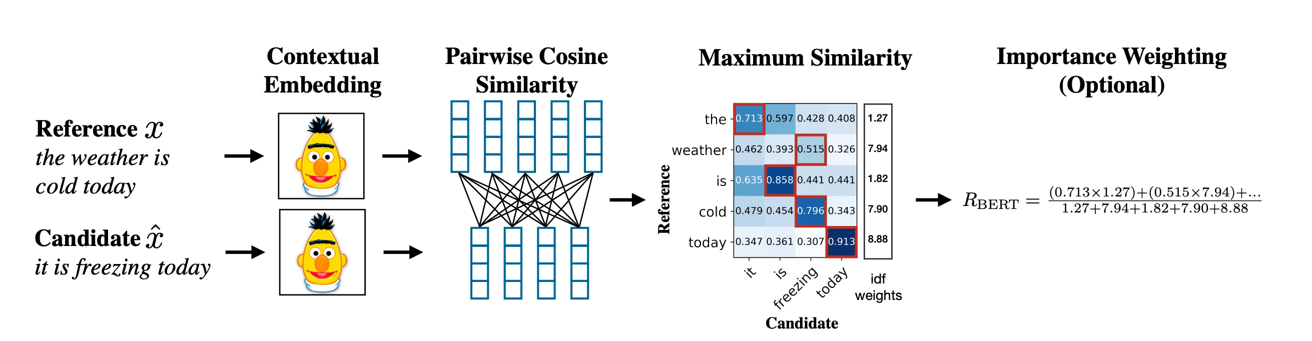
Image is from ‘Bertscore: evaluating text generation with bert’ by Tianyi Zhang et al, https://arxiv.org/pdf/1904.09675, page 4.
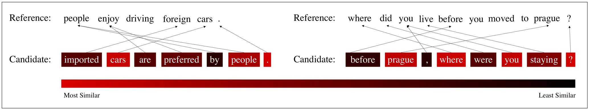
Image is from ‘Bertscore: evaluating text generation with bert’ by Tianyi Zhang et al, https://arxiv.org/pdf/1904.09675, page 16
BERTScore, like other embedding-based metrics, might sometimes struggle with evaluating the fluency or grammaticality of generated text. It might also be computationally expensive compared to simpler metrics like BLEU.
In addition to translation and image captioning, BERTScore is used for a veriety of evaluations, including evaluating text summarization, dialogue generation, and other natural language generation tasks.
In summary, BERTScore’s key innovation is the use of contextual embeddings (like those from BERT), which capture the specific use of a token in a sentence. This is a crucial difference from simpler word embeddings (earlier methods like MEANT 2.0 and YISI-1). BERTScore employs greedy matching to pair tokens between the candidate and reference sentences.
Further Reading:
SEM Score
It is semantic similarity between ground truth and model’s generation using an embedding model. It addresses the limitations of manual evaluation (time-consuming, not scalable) and traditional automated metrics (like BLEU and ROUGE, which rely on n-gram overlap and may not correlate well with human judgment, especially for instruction-tuned models). SEMScore was developed in this paper in February 2024.
SEMSCORE directly compares the semantic meaning of a model’s output to a gold target response. It uses sentence embeddings generated by a pre-trained sentence transformer (specifically, all-mpnet-base-v2 in the 2024 paper https://arxiv.org/pdf/2401.17072) for both the model response and the target response. The similarity between these embeddings is then calculated using cosine similarity, resulting in the SEMSCORE value (between -1 and 1). The authors evaluated SEMSCORE against 8 other widely-used text generation metrics on the outputs of 12 prominent instruction-tuned LLMs. They found that SEMSCORE exhibited the highest correlation with human evaluations compared to all other metrics, including more complex LLM-based metrics in many cases. G-Eval and BERTScore also showed strong correlations, while BLEU and ROUGE-L showed moderate correlations.
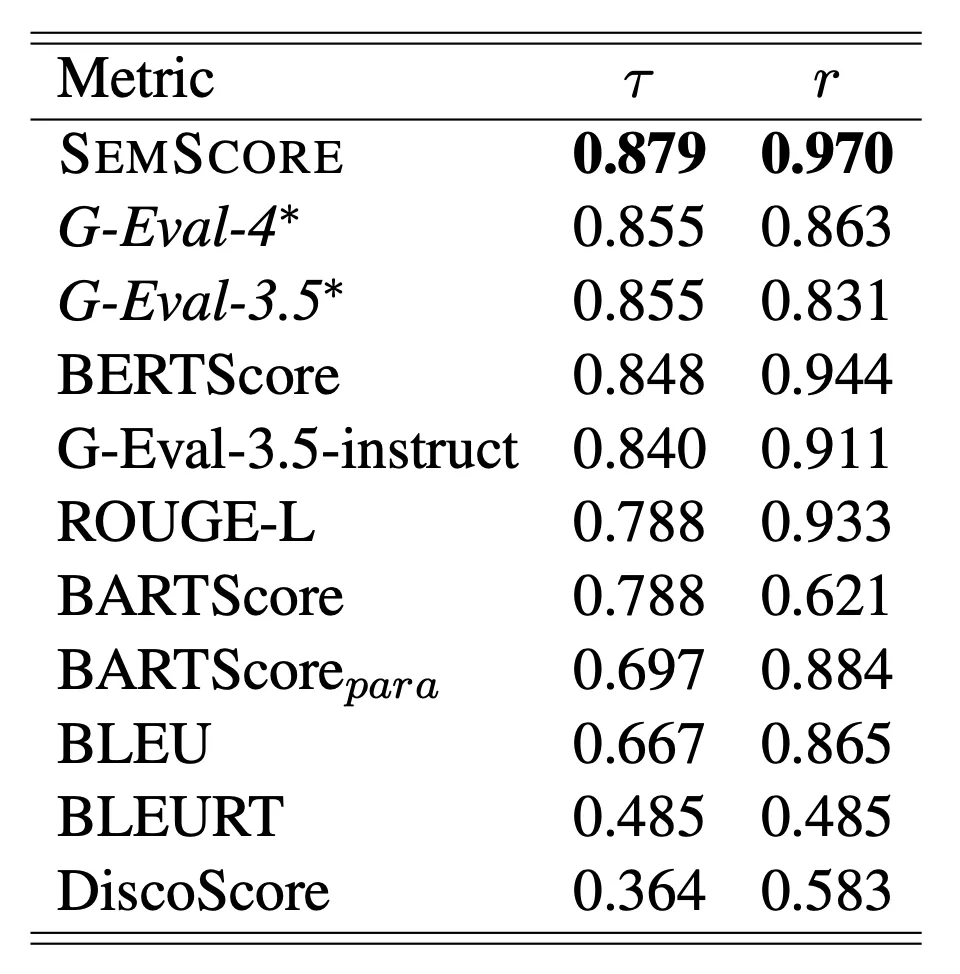
Table is from ‘SEMSCORE: Automated Evaluation of Instruction-Tuned LLMs based on Semantic Textual Similarity’ by Ansar Aynetdinov and Alan Akbik, https://arxiv.org/pdf/2401.17072 page 4
How SEMScore works:
- Embed Model and Target Response: The response generated by the Large Language Model (LLM) and the gold-standard target response (the desired output) is converted into a sentence embedding using a sentence transformer model.
- Calculate Cosine Similarity: The cosine similarity between the two sentence embeddings (the one from the model response and the one from the target response) is computed.
The resulting cosine similarity value is the SEMSCORE. This value ranges from -1 to 1, where a value closer to 1 indicates higher semantic similarity between the model’s response and the target response.
Advantages:
- High Correlation with Human Judgment: It better aligns with how humans perceive the quality of generated text.
- Simplicity: It’s a straightforward method to implement.
- Reproducibility: It doesn’t rely on proprietary models like GPT-4 or complex prompt engineering.
- Cost-Effective: It doesn’t incur the costs associated with using large language models for evaluation.
Limitations:
- Requirement of Gold Target Response: Like many other evaluation metrics, SEMSCORE needs at least one human-created or vetted target response for comparison.
- Dataset Size and Focus: The evaluation was conducted on a dataset that, while relevant for instruction-tuned LLMs, was relatively small and focused on a broad range of tasks rather than traditional NLP tasks.
The performance of SEMSCORE relies on the quality of the underlying sentence embedding model. The paper recommends using all-mpnet-base-v2.
At first glance, SEMScore may appear to be a generic embedding-based similarity algorithm, comparable to BERTScore. While this is largely accurate, there are several fundamental distinctions between SEMScore and BERTScore. SEMScore operates on the sentence/passage level by creating a single embedding for the entire text, while BERTScore works at the token level by computing similarities between individual tokens. Due to its sentence-level approach, SEMScore is more computationally efficient than BERTScore, which requires token-by-token comparisons. SEMScore is conceptually simpler and easier to implement, requiring just two straightforward steps (embedding and cosine similarity), compared to BERTScore’s more complex token alignment and weighting procedures. Despite using a smaller transformer model, SEMScore slightly outperforms BERTScore in correlating with human judgment of instruction-following quality.
Further Reading:
LLM-Based Evaluation
Using LLMs to judge quality from a human-like perspective.
In a RAG system, an LLM generates responses that are informed by external documents retrieved from a knowledge base, thereby enhancing the model’s ability to provide up‐to‐date or domain-specific information. Evaluating the quality of these responses can be challenging because traditional metrics (like BLEU or ROUGE) often miss nuances such as factual correctness or contextual coherence.
LLM‐based evaluation in RAG addresses these challenges by using an LLM as a “judge” for the generated outputs. Instead of relying solely on surface-level word overlaps, the evaluator LLM is prompted—often with chain‐of‐thought (CoT) techniques and few-shot examples—to reason through the quality dimensions of an output (e.g., correctness, relevance, readability, and comprehensiveness) and assign scores accordingly. This method can more closely mimic human judgment, enable rapid, automated evaluations, and help fine-tune and benchmark RAG systems in a scalable and cost-effective way.
Reference-Based vs Reference-Free Evaluation
LLM-Based evaluation is can be used reference-free, (a unique trait of this method) meaning a human is not needed to create samples. This is the major strength of this method. (Dicussed in this 2024 paper by Haitao Li et al https://arxiv.org/pdf/2412.05579, page 8)
Reference-Free Evaluation, in contrast, doesn’t rely on specific references but instead evaluates based on intrinsic quality standards or alignment with the source context. This method employs internal grammatical and semantic knowledge to assess factors like language fluency or content coherence. Its main advantage is flexibility for open-ended tasks, though it struggles in domains where the evaluator lacks relevant knowledge.
That being said, LLM-Based evaluation can also be used with references. Reference-Based Evaluation leverages reference data to determine whether performance meets expected standards. It’s commonly applied in Natural Language Generation tasks where output quality can be objectively judged by similarity to established references, such as in machine translation or text summarization. While this approach offers a well-defined benchmarking process, its effectiveness may be constrained by the quality and variety of the reference data available.
G-Eval
G‑Eval is a specific framework for evaluating natural language generation (NLG) outputs using LLMs—most notably, models such as GPT‑4. Its key innovation lies in these components:
- Prompt for NLG Evaluation: Natural language instructions defining the evaluation task and criteria
- Chain-of-Thought Reasoning: G‑Eval first generates a set of evaluation steps (or “reasoning instructions”) via an auto CoT process. These steps break down the evaluation task (for example, judging the coherence of a summary) into interpretable sub-tasks.
- Scoring Function with Form-Filling Paradigm: G-EVAL uses a form-filling approach where, after generating CoT steps, the LLM evaluates the text against clear criteria (e.g., “Coherence: 1-5”) and produces not just discrete scores but fine-grained continuous ratings by calculating a probability-weighted summation of possible scores, allowing it to capture subtle quality differences that integer-only ratings would miss.
G-EVAL is reference-free, which is a significant advantage over traditional metrics like BLEU and ROUGE that require reference outputs. This low reliance on human-annotated reference texts makes G-EVAL more scalable and applicable in scenarios where obtaining high-quality references is expensive, time-consuming, or even infeasible.
Addressing Common Issues
G-EVAL solves two common problems with direct scoring:
- Dominance of certain scores (e.g., 3 on a 1-5 scale)
- Integer-only scores that lead to many ties
By taking a probability-weighted summation of possible scores, G-EVAL produces more fine-grained, continuous scores. This means using the raw token probablities instead of querrying the model many times.
Effect of Model Size
- G-EVAL-4 (GPT-4 based) outperforms G-EVAL-3.5 (GPT-3.5 based) on most dimensions and datasets
- The improvement is more significant for challenging tasks like consistency and relevance
- On the simpler Topical-Chat benchmark, G-EVAL-3.5 and G-EVAL-4 perform similarly
Bias Toward LLM-Generated Outputs
G-Eval may have a bias towards LLM-generated texts, even when human evaluators prefer human-written content. This raises concerns about self-reinforcement if these evaluators are used as reward functions for further LLM training. G-EVAL-4 consistently gives higher scores to GPT-3.5 summaries than human-written ones, even when humans prefer the latter.
Conclusion
Empirical studies have shown that G‑Eval yields evaluations that correlate more strongly (compared with BLEU, ROUGE, METEOR, BertScore, ect) with human judgments (for instance, attaining Spearman correlations around 0.514 on summarization tasks) than traditional automatic metrics. This makes G‑Eval a powerful and flexible tool for assessing NLG quality—not only in standard text summarization but also across dialogue generation, question answering, and other RAG-based tasks.
Further Reading:
- G-Eval Paper: https://arxiv.org/abs/2303.16634
String-Level Similarity Checks
Non LLM string similarity is surface-level, based on matching of characters between two strings. These do not contain any language models. The most used non LLM string similarity algorithms are Levenshtein, Hamming, Jaro, and Jaro-Winkler.
- Levenshtein: based on the minimum number of single-character edits required to change one word into the other. See more by clicking here. Levenshtein distance is a type of edit distance — and when people say “edit distance,” they’re often referring to Levenshtein distance specifically. Edit distance is a general term: it’s the minimum number of operations needed to transform one string into another. Levenshtein distance is a specific kind of edit distance where the allowed operations are: insertion, deletion, and substitution.
- Hamming: looks at the number of positions in which the characters are different. See more by clicking here.
- Jaro: looks at the number of matching characters and number of transpositions required to get matching characters to align (given a strings in the correct order with only the characters in common.
- Jaro-Winkler: Jaro + increasing score if characters at the sart of both strings are the same — favouring same beginning. See more by clicking here.
Relevance Metrics
Is the generated answer or retrieved data relevant to the user’s query?
Response relevancy metrics evaluate how well an AI-generated answer or retrieved document aligns with the user’s query. Unlike traditional information retrieval metrics like precision and recall, these newer approaches focus specifically on measuring semantic alignment between queries and responses.
How Response Relevancy Works
The process follows an approach to measure semantic relevance:
- Question Generation: The system generates a set of artificial questions based on the content of the response. These questions are designed to capture the key information and topics covered in the response. This essentially reverses the Q&A process by creating questions that would naturally lead to the given response.
- Embedding Similarity Calculation: The system computes vector embeddings for both the original user input and each generated question. Embeddings capture the semantic meaning of text in a high-dimensional vector space. Cosine similarity is calculated between the user input embedding and each generated question embedding. This measures how semantically similar the response content is to what the user asked.
- Aggregation: The system takes the average of all cosine similarity scores to produce a final relevancy score. This provides a quantitative measure of how well the response addresses the user’s query.
The results is between -1 and 1, higher scores indicate greater relevance, and negative scores suggest the response may be addressing topics opposite to what was asked
Advantages:
- Captures semantic relevance rather than just lexical overlap
- Can detect relevant answers even when using different terminology than the query
- Less susceptible to keyword stuffing or other basic optimization techniques
Embedding Selection: The quality of embeddings dramatically affects measurement accuracy and speed. (FAISS, Annoy, ScaNN, HNSW)
These relevance metrics represent important advancements in evaluating AI system outputs, moving beyond traditional lexical matching toward deeper semantic understanding and multimodal context awareness. They help ensure that AI-generated content actually addresses what users are asking for, even when the relationship between query and response isn’t immediately obvious from surface-level text matching.
Conclusion
The diverse landscape of generative AI and RAG evaluation metrics includes various functions for each aspect of the AI system’s performance. These metrics can be categorized in multiple ways: by their technical implementation (such as simple string comparison algorithms, embedding-based methods, or LLM-based evaluations); by the quality they measure (including faithfulness, factualness, lexical similarity, and semantic similarity); by their computational complexity; by whether they require human input; or by their applicability to specific domains.
Table 2: Comparison of Retrieval Method Properties
| Metric / Method | Description | Needs Reference? | Method Type | Complexity | Correlation with Human Evaluation |
|---|---|---|---|---|---|
| Precision@k | Proportion of the top‑k retrieved items that are relevant. | Yes | String-level / Simple Comparison | Low | High in well‑defined retrieval settings |
| Recall@k | Proportion of relevant items that are retrieved among the top‑k results. | Yes | String-level / Simple Comparison | Low | High when relevance judgments are clear |
| F1@k | Harmonic mean of Precision@k and Recall@k. | Yes | String-level / Simple Comparison | Low | High (inherits behavior from precision and recall) |
| Mean Reciprocal Rank (MRR) | Average of the reciprocal ranks of the first relevant items across queries. | Yes | String-level / Simple Comparison | Low | Moderate to high depending on ranking sensitivity |
| Mean Average Precision (MAP) | Average of precision scores calculated after each relevant result is retrieved, averaged over all queries. | Yes | String-level / Simple Comparison | Medium | High in scenarios with well‑annotated ground truth |
| DCG@k / NDCG@k | Discounted (and normalized) cumulative gain; accounts for relevance and rank position. | Yes | String-level / Logarithmic Discounting | Medium | High if user satisfaction can be approximated by rank decay |
| Expected Reciprocal Rank (ERR) | Models user behavior to estimate the expected reciprocal rank based on graded relevance. | Yes | String-level / Probabilistic Model | Medium-High | Generally high when the user’s examination model is realistic |
Table 3: Comparison of Generation Evaluation Methods
| Metric / Method | Description | Needs Reference? | Method Type | Complexity | Correlation with Human Evaluation |
|---|---|---|---|---|---|
| BLEU | N‑gram overlap metric that compares candidate text to one or more reference texts (commonly used in MT evaluation). | Yes | String-level / N‑gram Matching | Low | Moderate; known to sometimes poorly capture nuanced human judgment |
| ROUGE | Measures recall of n‑gram overlap between candidate and reference summaries. | Yes | String-level / N‑gram Matching | Low | Moderate; can be effective for summarization, though sometimes insensitive |
| METEOR | Considers exact, stem, synonym, and paraphrase matches between candidate and reference. | Yes | String-level / N‑gram + Synonym Matching | Medium | Moderate to high; often improves on BLEU/ROUGE by better aligning to human views |
| HHEM (Hallucination Evaluation Metric) | Designed to detect hallucinations (unfaithful content) in generated text. | Optional (Reference‑free approaches exist) | LLM-based / Specialized Evaluation | High | High when tuned for hallucination detection, though still under active research |
| Factual Correctness | Evaluates whether the generated text aligns with known facts. | Optional (can be reference‑free, e.g., via fact‑checking) | Embedding-based / LLM-based evaluation | High | Moderate to high, but results vary with implementation and domain |
| BERTScore | Compares contextual embeddings between candidate and reference texts using BERT representations. | Yes | Embedding-based | Medium | Generally high; often correlates well with human judgments in semantic tasks |
| SEM Score | Another semantic embedding–based metric assessing similarity on a deeper level. | Yes | Embedding-based | Medium (simpler than BERTScore) | High, depending on embedding quality and domain |
| G-Eval | Leverages large language models (LLMs) to evaluate texts across multiple axes (fluency, relevance, etc.). | No (can be reference‑free) | LLM-based | High | Promising but variable; early studies suggest decent alignment with human ratings |
| String-Level Similarity Checks | Basic checks for exact or partial matches using string comparison algorithms. | Yes | String-level | Low | Low; does not capture subtleties of meaning, so weaker correlation |
| Relevance Metrics | Quantifies how closely a generated response fits the intended user query and context. | Optional (depending on if a reference context exists) | LLM-based / Embedding-based evaluation | Medium | Moderate; effectiveness depends on task formulation and user criteria |
| Relevance Metrics | Quantifies how closely a generated response fits the intended user query and context. | Optional (depending on if a reference context exists) | LLM-based / Embedding-based evaluation | Medium | Moderate; effectiveness depends on task formulation and user criteria |
Understanding the available evaluation techniques and their attributes is essential for selecting the most appropriate metrics tailored to each specific case and situation. This ensures accurate assessment of system performance and alignment with project objectives.
Automated metrics provide quick, scalable insights, yet they can overlook nuances captured only by human judgment. Metrics are proxies, and human judgment helps validate them. The goal is to achieve higher human correspondence, while taking into account factors like text type, cost, speed, and scalability, ensuring that the solution is not only effective but also efficient and practical in real-world applications.